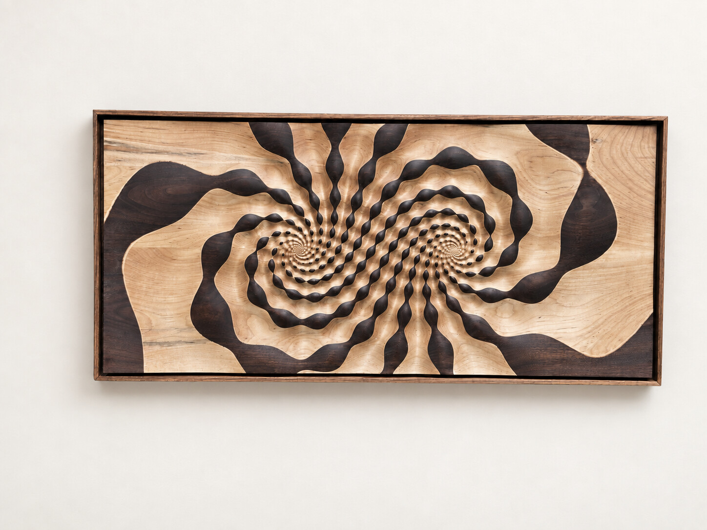
Using a loxodromic transformation to generate form.

It is appropriate that things different in substance, but alike in form, should be put into the same mold, so to speak. When our language is well chosen, it is astonishing to see how all the demonstrations made upon some known fact immediately become applicable to many new facts. Nothing has to be changed, not even the words, since the names are the same in the new cases.
- Henri Poincaré

These notes are an exploration of the mathematics, design, and craft behind a carved wall panel for Yale's Mathematics Department. They record the process of designing the Loxodromic Panel using the mathematics of the complex plane and ask how a loxodromic transformation can become a periodic carved height field.

The aim is to build and design directly using math and to produce an artifact that is beautiful in its own right.

The Problem

The goal of this project is to produce a 3D representation of a loxodromic transformation like the one shown here.

Computed trajectories of the loxodromic flow. The left fixed point repels forward orbits; the right fixed point attracts them.

We don't want to just show invariant curves like in the image above, but rather to express the operation of function application: what does the transformation do?

So, rather than just have ridges where the invariant curves are, the idea is to show regions that follow along the invariant curves but vary their thickness. This produces a series of bulges, and applying the loxodromic transformation carries each bulge to the next one along its curve.

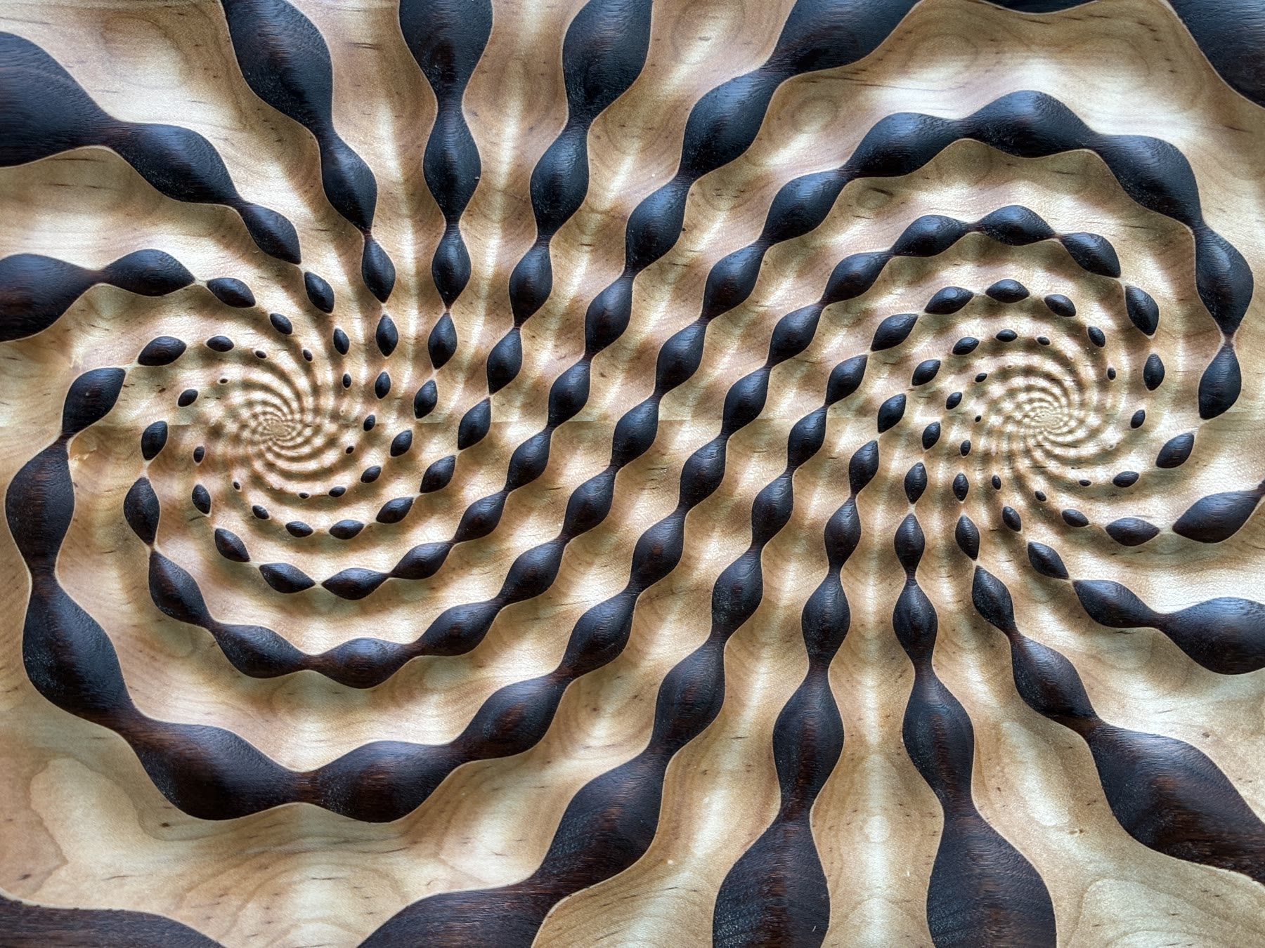
The completed Loxodromic Panel, with alternating walnut and maple bulges spiraling toward two fixed points. — The completed Loxodromic Panel, made for Yale's Mathematics Department.

We'll start by generating the transformation.

The Transformation

A loxodromic Möbius transformation has two fixed points and, in suitable coordinates, acts by a dilation together with a rotation. Here we are interested in transformations for which both the dilation and the rotation are nontrivial.

The transformation we're seeking in the panel plane has two fixed points at $\pm i$ . We extend the plane to the Riemann sphere by adjoining a point at infinity, then choose a coordinate in which the fixed points are $0$ and $\infty$ . Call the panel coordinate $p$ and the new coordinate $z$ . These are two coordinates on the same sphere, related by

z=M(p)=\frac{p+i}{p-i},\qquad p=M^{-1}(z)=i\,\frac{z+1}{z-1}.

\begin{aligned}z&=M(p)=\frac{p+i}{p-i},\\p&=M^{-1}(z)=i\,\frac{z+1}{z-1}.\end{aligned}

This sends $p=-i$ to $z=0$ and $p=i$ to $z=\infty$ . In the $z$ -coordinate, our transformation is simply

L(z)=\gamma z,\qquad \gamma=1.9e^{i\pi/3}.

\begin{aligned}L(z)&=\gamma z,\\\gamma&=1.9e^{i\pi/3}.\end{aligned}

I chose this value of $\gamma$ by experimentation. Each application multiplies the distance from the origin by $1.9$ and rotates by $\pi/3$ . In the panel coordinate, the corresponding transformation in the p-plane is $M^{-1}\circ L\circ M$ .

A natural family of invariant curves consists of logarithmic spirals. Let

\lambda=\operatorname{Log}\gamma=\ln(1.9)+\frac{\pi i}{3}.

For example, the spiral through $1$ can be parametrized as

z(u)=e^{u\lambda},\qquad u\in\mathbb{R}.

Applying $L$ to a point on this spiral is equivalent to increasing $u$ by $1$ :

\begin{aligned}L(z(u))&=\gamma e^{u\lambda}\\&=e^{(u+1)\lambda}\\&=z(u+1).\end{aligned}

The Snakes

One application of the transformation is a translation by $1$ in $u$ . To introduce neighboring snakes, we add a second coordinate, $v$ , and move perpendicular to the $u$ -direction in a new plane:

w=u+iv,\qquad z(w)=e^{\lambda w}.

\begin{aligned}w&=u+iv,\\z(w)&=e^{\lambda w}.\end{aligned}

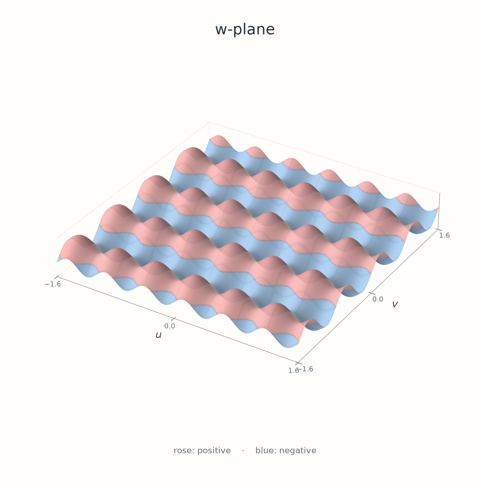
Each horizontal line $v=v_0$ maps to a logarithmic spiral, and increasing $u$ moves along it. To generate the bulges, start with a periodic field in this plane:

h_W(u+iv)=\sin(8v)+\frac12\sin(12u).

\begin{aligned}h_W(u+iv)&=\sin(8v)\\&\quad+\frac12\sin(12u).\end{aligned}

The two terms have periods $\pi/4$ in $v$ and $\pi/6$ in $u$ . These frequencies were an initial visual choice. We will see what happens when the field is carved.

Perspective graph of sin(8v) plus one half sin(12u) in the w-plane, with rose positive heights and blue negative heights. — The initial height field in the $w=u+iv$ plane. Rose marks positive height; blue marks negative height.

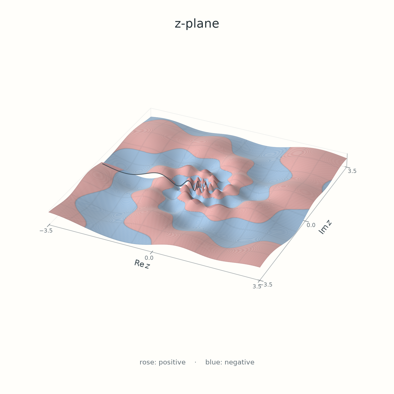
Before mapping this height field into the $z$ -plane, we need a computational technique for evaluating it on the panel.

Computation

For fabrication, we need heights at the points sampled by the panel mesh. We can start with those points in the panel plane and transform each one into the $z$ -plane, then into the $w$ -plane, where the height is easy to calculate. Here I'm taking extra care to distinguish the variious spaces in which height is calculated. $p$ is the panel coordinate, $z$ is the complex plane where $0$ and $\infty$ are fixed, and $w$ is the rectilinear periodic coordinate. The coordinate relationships are

z=M(p),\qquad z=e^{\lambda w}.

\begin{aligned}z&=M(p),\\z&=e^{\lambda w}.\end{aligned}

To choose one inverse value, we use the principal logarithm, denoted by $\operatorname{Log}$ , whose argument lies between $-\pi$ and $\pi$ on the slit plane. Then

w=\frac{\operatorname{Log}z}{\lambda},\qquad h_Z(z)=h_W\!\left(\frac{\operatorname{Log}z}{\lambda}\right).

\begin{aligned}w&=\frac{\operatorname{Log}z}{\lambda},\\h_Z(z)&=h_W\!\left(\frac{\operatorname{Log}z}{\lambda}\right).\end{aligned}

The same initial height field pulled into the z-plane using the principal logarithm, accumulating toward zero. — The same field in the $z$ -plane. Its oscillations crowd toward $z=0$ ; the open edge along the negative real axis will matter when we carve it.

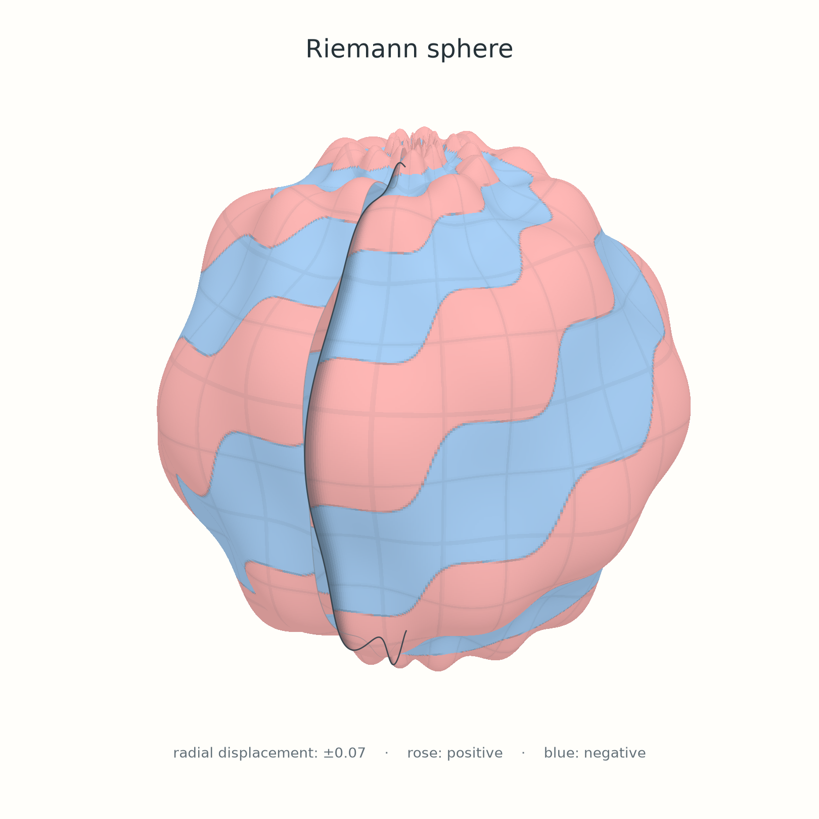
We can also view the $z$ -plane as the Riemann sphere by inverse stereographic projection. Here the same scalar height is shown as a small radial displacement of a unit sphere. The displacement is a drawing convention, not another coordinate transformation.

R(z)=1+0.03\,h_Z(z).

The same height field displayed as a small radial deformation of the Riemann sphere, with the branch-cut seam visible. — On the Riemann sphere, $z=0$ and $z=\infty$ are the two poles. The open line marks the edges of the coordinate cut, not a feature of the sphere itself.

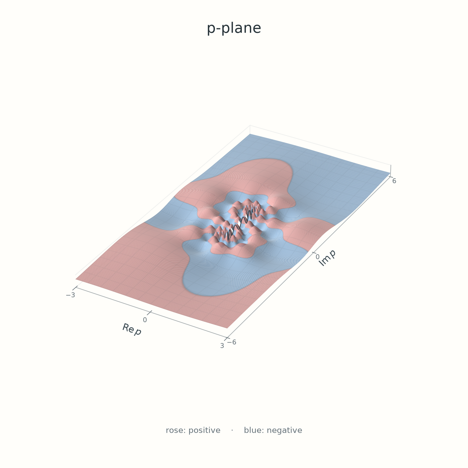
The height assigned to a point on the panel is therefore

\begin{aligned}h_P(p)&=h_Z(M(p))\\&=h_W\!\left(\frac{\operatorname{Log}(M(p))}{\lambda}\right).\end{aligned}

The same field in the p-plane, with oscillations accumulating near the two fixed points at plus and minus i. — In the panel's $p$ -plane, the two accumulation points are $\pm i$ . The open edge runs along the segment joining them.

Fabrication

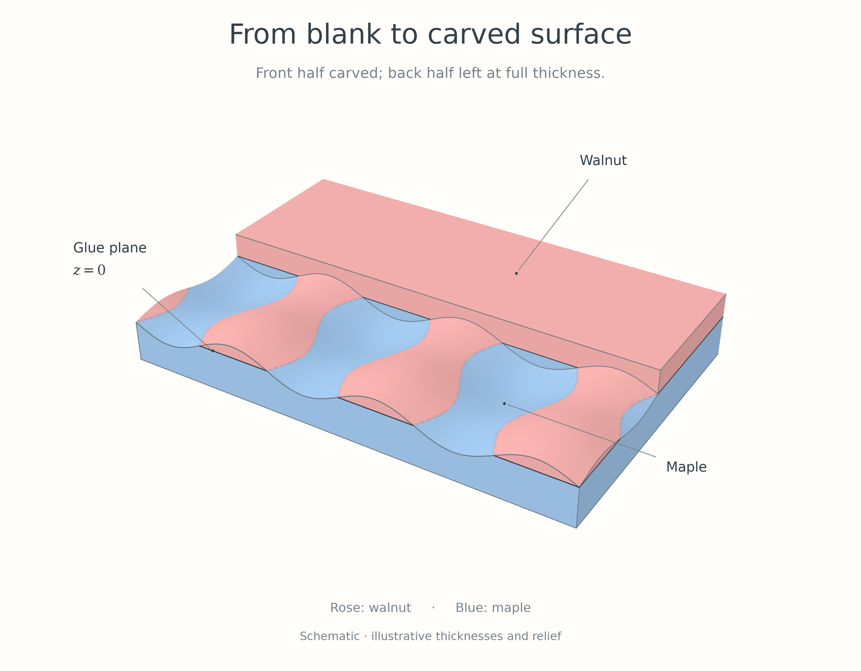
To acheive the two tone effect, I laminated a thin black walnut board on top of a lighter maple board. The, using a CNC router to translate the computed values into physical space, I carved the height field into the walnut. The depth of the cut determines how much walnut remains at the surface, and where the cut is deep enough to remove all the walnut, the maple shows through. The plane where the two species meet is where the function $h_P$ is zero.

Schematic laminated block with a flat, uncut walnut rear half and a carved front half that exposes maple where the surface falls below the glue plane. — A construction schematic: the front half is carved, while the back remains uncut. Rose represents walnut and blue represents maple; the layer thicknesses are illustrative.

The cutter makes repeated passes, removing material to the computed depth at each position. In the workshop footage, the spiral pattern gradually emerges from the laminated blank.

Three views of the carving process, condensed to nine seconds.

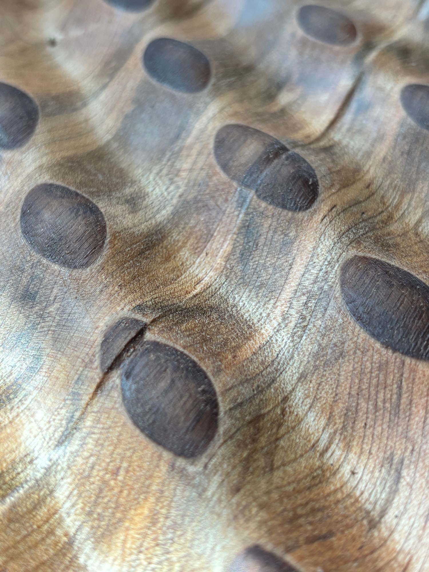
The first carved piece had a visible seam. The bulges on one side did not meet those on the other:

Close-up of the first carved piece, with a discontinuous seam cutting through the dark oval bulges. — The first piece, before the height field was adjusted to close the seam.

The router had followed the heights it was given. To understand the break, we had to return to the inverse map used to compute those heights.

Patching the Logarithmic Seam

The seam came from the principal logarithm in the inverse map. On the two sides of the negative real axis in the $z$ -plane, its limiting values differ by $2\pi i$ . Under $w=\operatorname{Log}z/\lambda$ , this becomes a jump in the coordinates at which we evaluate the height:

\Delta w=\frac{2\pi i}{\lambda}.

The inverse Möbius map $M^{-1}$ carries that cut to the segment between $-i$ and $i$ in the panel plane, exactly where the carving broke. There is no continuous single-valued logarithm on $\mathbb{C}^{\times}$ , so the logarithm itself cannot be repaired globally. Instead, we can patch the height field across its cut: make this coordinate jump a period of the field. Then both sides give the same height and matching derivatives.

h_W\!\left(w+\frac{2\pi i}{\lambda}\right)=h_W(w),\qquad w\in\mathbb{C}.

\begin{aligned}h_W\!\left(w+\frac{2\pi i}{\lambda}\right)&=h_W(w),\\w&\in\mathbb{C}.\end{aligned}

The initial frequencies did not satisfy this condition. Adjusting the two sine frequencies gives us two parameters to fit the logarithm's jump. Introduce nonzero real numbers $a$ and $b$ and set

h_W(u+iv)=\sin\!\left(\frac{8v}{a}\right)+\frac12\sin\!\left(\frac{12u}{b}\right).

\begin{aligned}h_W(u+iv)&=\sin\!\left(\frac{8v}{a}\right)\\&\quad+\frac12\sin\!\left(\frac{12u}{b}\right).\end{aligned}

For the first sine term, its argument must change by an integer multiple of $2\pi$ . Using $\operatorname{Im}(i\zeta)=\operatorname{Re}\zeta$ , we obtain

\begin{aligned}\frac8a\operatorname{Im}\!\left(w+\frac{2\pi i}{\lambda}\right)&=\frac8a\operatorname{Im}w+\frac{16\pi}{a}\operatorname{Re}\!\left(\frac1\lambda\right)\\&=\frac8a\operatorname{Im}w+2\pi m,\qquad m\in\mathbb{Z}.\end{aligned}

\begin{aligned}&\frac8a\operatorname{Im}\!\left(w+\frac{2\pi i}{\lambda}\right)\\&=\frac8a\operatorname{Im}w\\&\quad+\frac{16\pi}{a}\operatorname{Re}\!\left(\frac1\lambda\right)\\&=\frac8a\operatorname{Im}w+2\pi m,\\&\hspace{1em}m\in\mathbb{Z}.\end{aligned}

Thus the condition on the imaginary-coordinate term involves the real part of $1/\lambda$ :

\begin{aligned}\frac{16\pi}{a}\operatorname{Re}\!\left(\frac1\lambda\right)&=2\pi m,\\\operatorname{Re}\!\left(\frac1\lambda\right)&=\frac{am}{8}.\end{aligned}

For the second sine term, use $\operatorname{Re}(i\zeta)=-\operatorname{Im}\zeta$ . The same calculation gives

\begin{aligned}\frac{12}{b}\operatorname{Re}\!\left(w+\frac{2\pi i}{\lambda}\right)&=\frac{12}{b}\operatorname{Re}w-\frac{24\pi}{b}\operatorname{Im}\!\left(\frac1\lambda\right)\\&=\frac{12}{b}\operatorname{Re}w+2\pi n,\qquad n\in\mathbb{Z}.\end{aligned}

\begin{aligned}&\frac{12}{b}\operatorname{Re}\!\left(w+\frac{2\pi i}{\lambda}\right)\\&=\frac{12}{b}\operatorname{Re}w\\&\quad-\frac{24\pi}{b}\operatorname{Im}\!\left(\frac1\lambda\right)\\&=\frac{12}{b}\operatorname{Re}w+2\pi n,\\&\hspace{1em}n\in\mathbb{Z}.\end{aligned}

The condition on the real-coordinate term therefore involves the imaginary part of $1/\lambda$ , with a minus sign:

\begin{aligned}-\frac{24\pi}{b}\operatorname{Im}\!\left(\frac1\lambda\right)&=2\pi n,\\\operatorname{Im}\!\left(\frac1\lambda\right)&=-\frac{bn}{12}.\end{aligned}

These conditions give a family of possible frequency choices. Taking $m=8$ and $n=-12$ gives the choice used for the panel:

a=\operatorname{Re}\!\left(\frac1\lambda\right),\qquad b=\operatorname{Im}\!\left(\frac1\lambda\right).

\begin{aligned}a&=\operatorname{Re}\!\left(\frac1\lambda\right),\\b&=\operatorname{Im}\!\left(\frac1\lambda\right).\end{aligned}

With this choice, $1/\lambda=a+ib$ , so crossing from the lower bank to the upper bank changes $u$ by $-2\pi b$ and $v$ by $2\pi a$ . The sine arguments consequently change by $16\pi$ and $-24\pi$ : eight periods of the first sine and minus twelve periods of the second.

The height field therefore joins smoothly across the seam, even though the chosen $w$ -coordinates jump. It defines a smooth, single-valued function on $\mathbb{C}^{\times}=\mathbb{C}\setminus\{0\}$ . The oscillations still prevent a continuous extension to the two fixed points, $0$ and $\infty$ .

A new Transformation

Now that the seam is closed, we can ask which transformations preserve the resulting pattern. The original multiplier $\gamma$ corresponds to a translation by $1$ in the $u$ -direction. The new sine frequencies have their own periods, so a unit translation need not carry a bulge precisely to the next one. To find that transformation, we must use the actual periods of the height field.

The Symmetries

The symmetries are easiest to see in the $w$ -plane, where the pattern repeats on a rectangular lattice. For our choice of $\lambda$ , we have $a>0$ and $b<0$ . The positive periods in the two coordinate directions are

P_u=\frac{\pi|b|}{6}=-\frac{\pi b}{6},\qquad P_v=\frac{\pi a}{4}.

\begin{aligned}P_u&=\frac{\pi|b|}{6}=-\frac{\pi b}{6},\\P_v&=\frac{\pi a}{4}.\end{aligned}

A translation by $P_u$ advances one bulge along a horizontal row. A translation by $iP_v$ moves to the corresponding bulge in the neighboring row. Both preserve the entire height field:

h_W(w+P_u)=h_W(w),\qquad h_W(w+iP_v)=h_W(w).

\begin{aligned}h_W(w+P_u)&=h_W(w),\\h_W(w+iP_v)&=h_W(w).\end{aligned}

More generally, its translation periods are exactly

\Lambda=\{rP_u+siP_v:r,s\in\mathbb{Z}\}.

The two sine terms depend on independent coordinates, so a translation preserves the field everywhere precisely when each term returns to the same phase. This is why the periods form a rectangular lattice.

From a translation to a loxodromic transformation

Under the exponential map, adding any complex number $t$ to $w$ becomes multiplication in the $z$ -plane:

e^{\lambda(w+t)}=e^{\lambda t}e^{\lambda w}.

If $t\in\Lambda$ , this multiplication preserves the height field. Indeed, writing $z=e^{\lambda w}$ , we have

h_Z(e^{\lambda t}z)=h_W(w+t)=h_W(w)=h_Z(z).

\begin{aligned}h_Z(e^{\lambda t}z)&=h_W(w+t)\\&=h_W(w)\\&=h_Z(z).\end{aligned}

The seam calculation makes this identity valid independently of which logarithm we use to recover $w$ . Every other choice differs by an integer multiple of $2\pi i/\lambda$ , which is itself a period.

To move one bulge forward along its snake, take $t=P_u$ . The resulting transformation is

L_u(z)=\gamma_u z,\qquad \gamma_u=e^{\lambda P_u}.

\begin{aligned}L_u(z)&=\gamma_u z,\\\gamma_u&=e^{\lambda P_u}.\end{aligned}

With $\gamma=1.9e^{i\pi/3}$ , these values are

\begin{aligned}P_u&\approx0.363457,\\\gamma_u&\approx1.262743\,e^{0.380612i}. \end{aligned}

Thus one step scales distance from the origin by about $1.263$ and rotates by about $21.81^{\circ}$ . Each horizontal line still maps to the same logarithmic spiral as before, but we now advance by $P_u$ along that line. The original multiplier determines the spiral family; the height field determines the step that repeats the bulges.

The original map $z\mapsto\gamma z$ advances by $1$ . Here $1/P_u$ is not an integer, so that step does not preserve the height field. This is the precise sense in which the finished pattern visualizes a different loxodromic transformation.

Returning to the panel

The corresponding transformation in the panel coordinate is obtained by conjugating with $M$ :

\begin{aligned}T_u(p)&=M^{-1}\!\bigl(\gamma_u M(p)\bigr)\\&=i\,\frac{(\gamma_u+1)p+i(\gamma_u-1)}{(\gamma_u-1)p+i(\gamma_u+1)}. \end{aligned}

It fixes $\pm i$ and satisfies

h_P(T_u(p))=h_P(p),\qquad p\in\widehat{\mathbb{C}}\setminus\{-i,i\}.

\begin{aligned}h_P(T_u(p))&=h_P(p),\\p&\in\widehat{\mathbb{C}}\setminus\{-i,i\}.\end{aligned}

This equation expresses the design goal: applying the transformation carries each bulge to the next bulge along its curve, with the same height at corresponding points. Repeated forward applications approach $p=i$ , while repeated inverse applications approach $p=-i$ . The bulges become progressively smaller in the plane as they approach either fixed point.

The symmetry is a property of the ideal scalar height field. Its graph is preserved by mapping $p$ to $T_u(p)$ and keeping the height coordinate unchanged. This map is not a rigid motion in three-dimensional Euclidean space, and the rectangular crop used for the physical panel is a separate design choice.

The family of multiplication symmetries

Moving along a snake is one symmetry among many. Every lattice period gives a multiplier

\gamma_{r,s}=e^{\lambda(rP_u+siP_v)},\qquad r,s\in\mathbb{Z}.

Here we are considering the Möbius symmetries that fix $0$ and $\infty$ individually, so they have the form $z\mapsto qz$ . Every such symmetry comes from a period of $h_W$ , but distinct periods need not give distinct transformations. The exponential map identifies

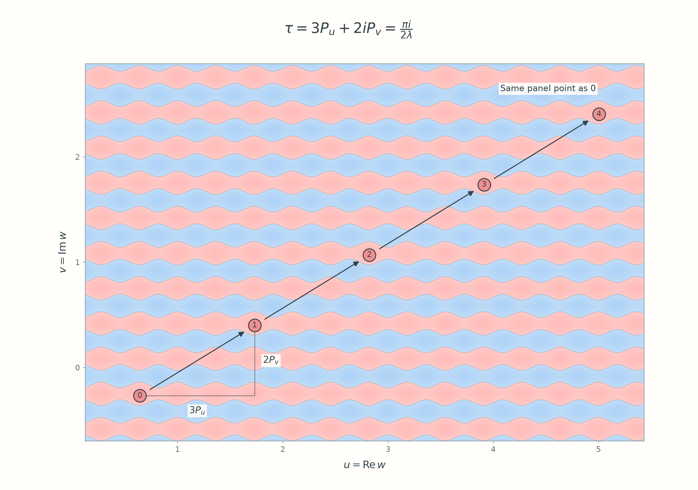
w\sim w+\frac{2\pi i}{\lambda},\qquad \frac{2\pi i}{\lambda}=12P_u+8iP_v.

\begin{aligned}w&\sim w+\frac{2\pi i}{\lambda},\\\frac{2\pi i}{\lambda}&=12P_u+8iP_v.\end{aligned}

Consequently, twelve horizontal steps followed by eight vertical steps return to exactly the same point in the $z$ -plane. Integer pairs $(r,s)$ describe the same multiplier precisely when they differ by an integer multiple of $(12,8)$ . Quotienting the lattice by this relation gives the group of multiplication symmetries:

G\cong\Lambda\big/\left(\frac{2\pi i}{\lambda}\mathbb{Z}\right)\cong\mathbb{Z}^2/\langle(12,8)\rangle\cong\mathbb{Z}\oplus\mathbb{Z}/4\mathbb{Z}.

\begin{aligned}G&\cong\Lambda\big/\left(\frac{2\pi i}{\lambda}\mathbb{Z}\right)\\&\cong\mathbb{Z}^2/\langle(12,8)\rangle\\&\cong\mathbb{Z}\oplus\mathbb{Z}/4\mathbb{Z}.\end{aligned}

The factor of four has a direct geometric meaning. A quarter of the logarithm's period is already a period of the height field:

3P_u+2iP_v=\frac{\pi i}{2\lambda},\qquad e^{\lambda(3P_u+2iP_v)}=i.

\begin{aligned}3P_u+2iP_v&=\frac{\pi i}{2\lambda},\\e^{\lambda(3P_u+2iP_v)}&=i.\end{aligned}

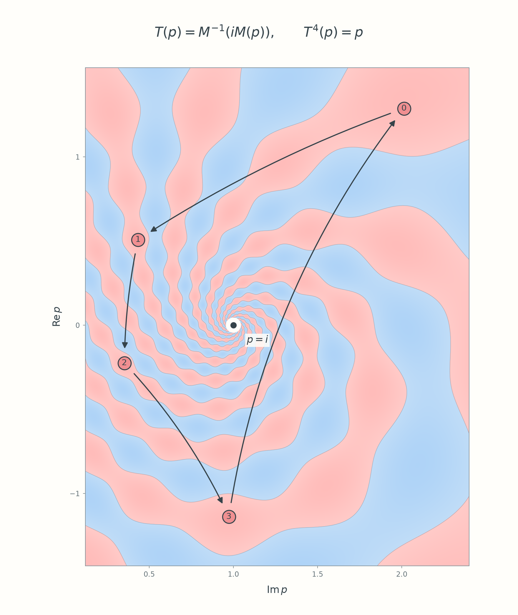
Rose and blue height field in the w-plane with five numbered points joined by equal diagonal translation arrows. Each step moves three horizontal periods and two vertical periods; point four maps to the same panel point as point zero. — In the $w$ -plane, each arrow translates by $\tau=3P_u+2iP_v$ . Points 0–3 correspond to the four marked bulges in the panel diagram below. After four steps, the displacement is $2\pi i/\lambda$ : point 4 is distinct from point 0 here, but exponentiation sends them to the same $z$ , and hence the same panel point.

Hence $h_Z(iz)=h_Z(z)$ : the field has a fourfold rotational symmetry about the two poles. On the Riemann sphere this is a rotation by $90^{\circ}$ . In the panel plane, call the corresponding order-four Möbius transformation $T(p)=M^{-1}(iM(p))$ .

Top-down close-up of the rose and blue panel height field near p equals i, with four numbered dots on bulges and arrows showing their order-four Möbius correspondence. — Near one fixed point, $T$ sends each numbered bulge to the next; the fourth step returns to the start. The arrows show discrete correspondences, not paths of motion or a rigid rotation of the panel.

The source code for these diagrams is public, including the coordinate-space plots, construction schematics, and both symmetry diagrams. The CNC mesh generator is a separate program.

Straight-on close view of the finished panel, showing walnut and maple curves winding into the two spiral centers. — The finished panel. The walnut and maple boundary makes the field visible, and the relief changes how it catches the light.

Special thanks to Yair Minsky for helping me clarify the seam-fixing calculations.